Spin-magnetic calculation in Quantum ESPRESSO

In this tutorial, we walk you through the steps of spin magnetic bandstructure calculation using Quantum Espresso on our web platform.

1. Specify material structure

First of all, to perform material simulation, we need to specify the material structure. We can create a new material on our platform using Materials Designer. Alternatively, we can upload structure files (e.g., CIF, or VASP POTCAR format), or import materials from the Materials bank in Mat3ra platform.

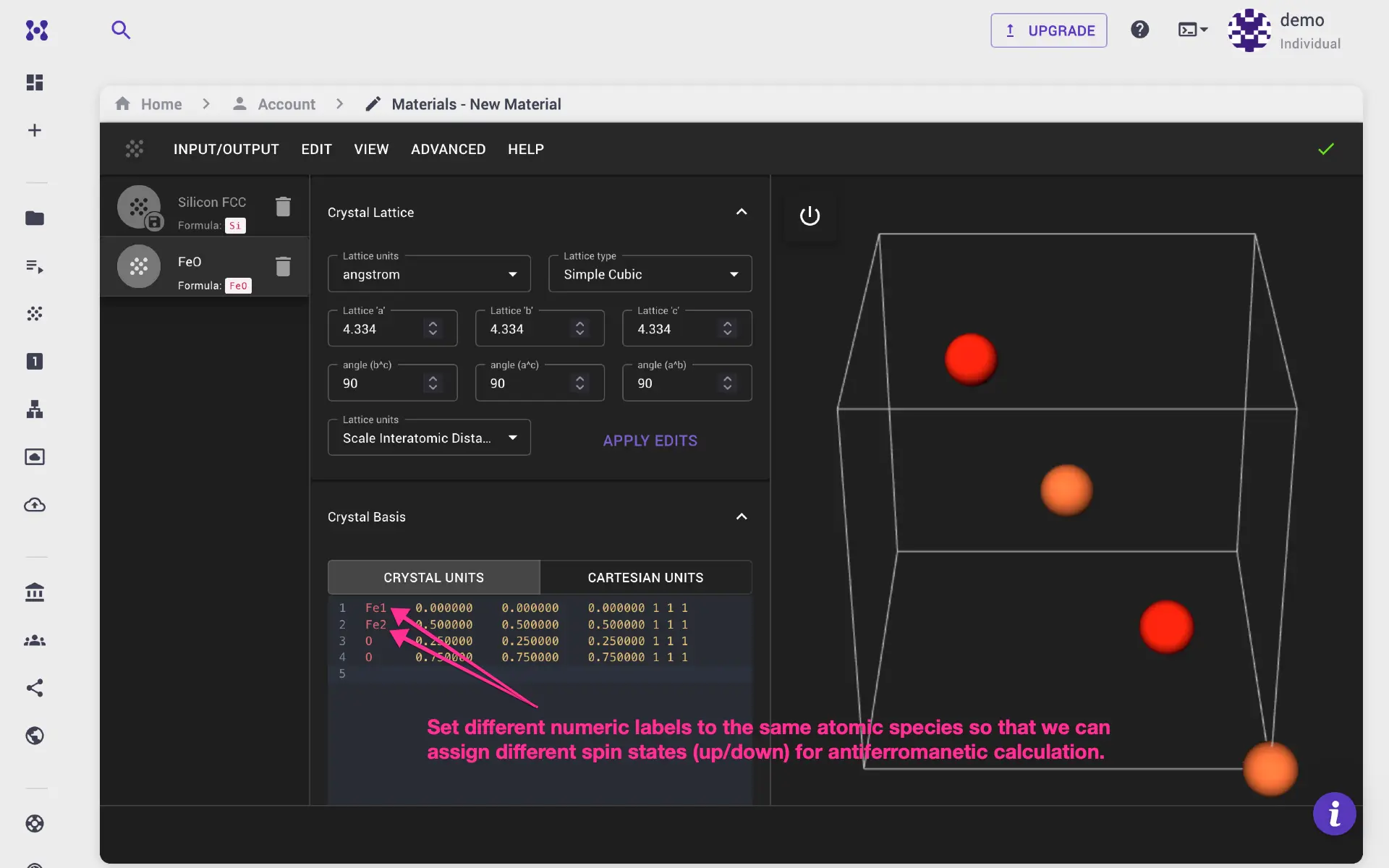
Notice, that if we want to assign different spin states (i.e., up or down) to the same atomic species, we must add numeric labels to the atomic symbols. In this case, the unit cell has two Fe atoms, we added Fe1 and Fe2 labels.

2. Create workflow

Below we will show how to create a workflow for spin magnetic bandstructure calculation. Alternatively, you may find the desired workflow in the workflow bank on our platform, and you can import it to your library/account. Our example calculation involves three steps:

1. Perform self-consistent field (SCF) calculation
2. Perform bands (NSCF) calculation along specific k-path
3. Post-processing of bands calculation

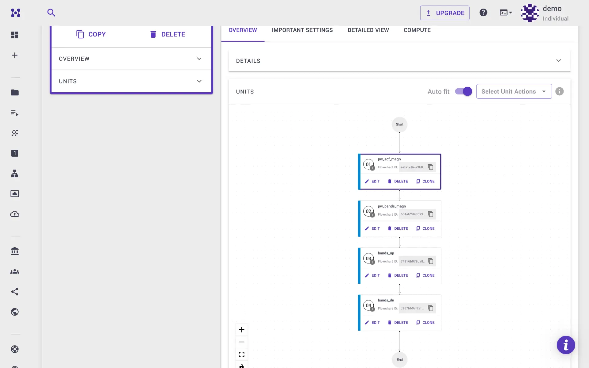
2.1. SCF workflow unit

There are several templates for spin magnetic calculation. Here we choose pw_scf_magn. If you like to perform DFT+U, DFT+U+V, or DFT+U+J in conjunction with spin-polarization, please select the respective template.

2.2. Bands calculation

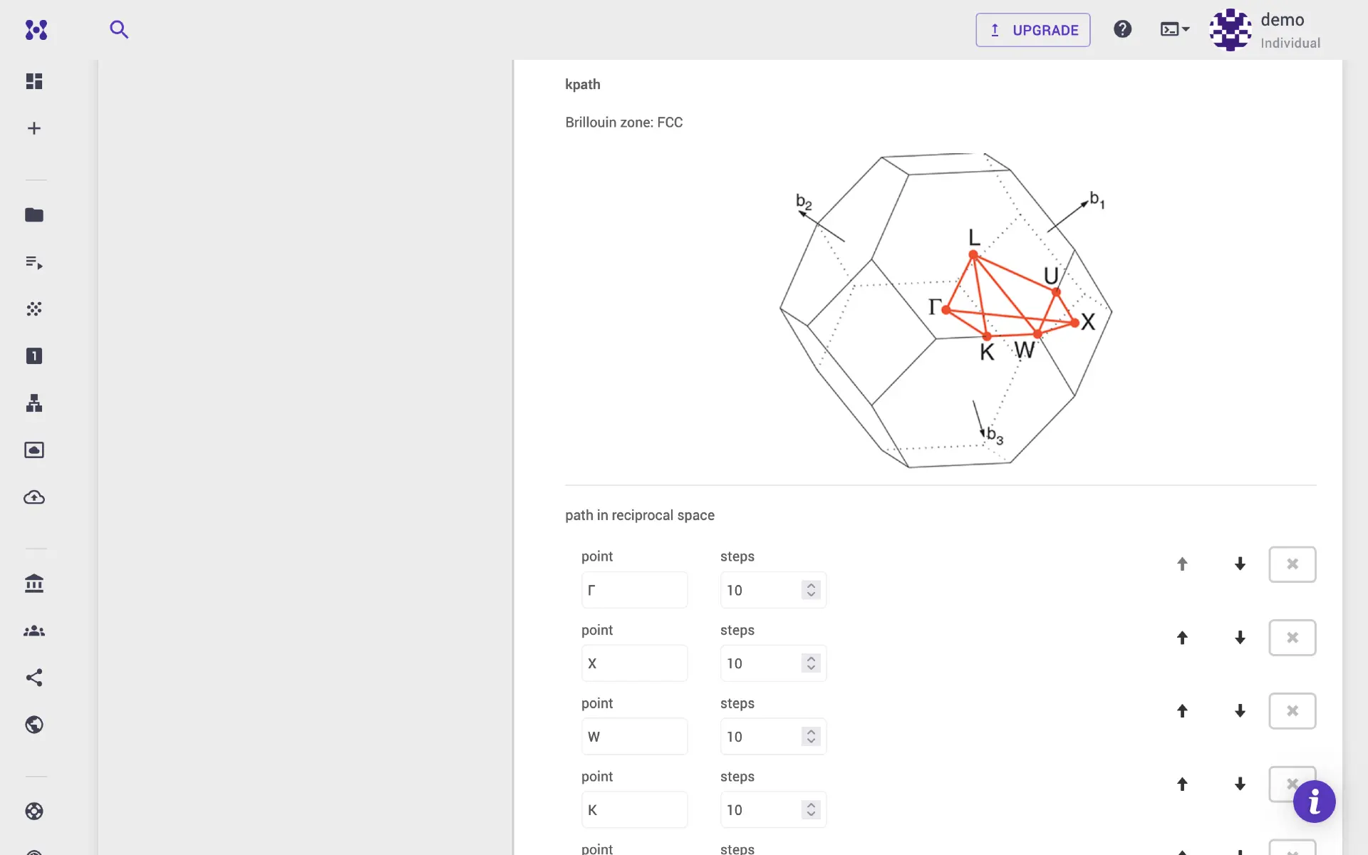
In the next step, we add a unit for bands calculation and select pw_bands_magn template. This performs nscf calculation along the specified k-path. We can set the desired k-path via the Important Settings tab.

2.3. Bands.x postprocessing

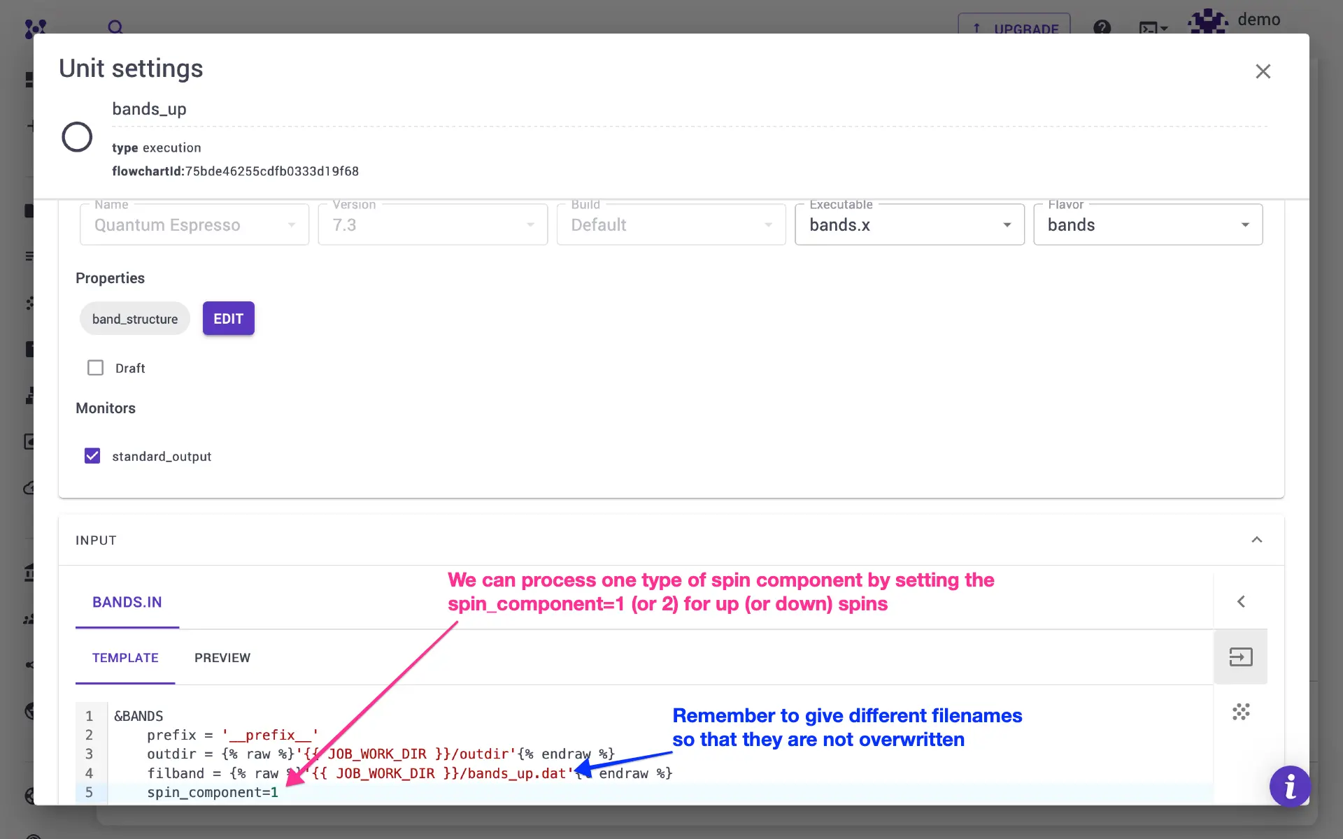
In the final step, we add bands.x calculation. This step is optional, and used for further postprocessing of already calculated bandstructure data in the above steps. We are interested in processing one type of spin (i.e., up or down) state. We can do that by specifying spin_component = 1 for up spin, or spin_component = 2 for down spin. So we add two units, one to process only up and another to process down spin only. We update the filbands filenames so that the outputs are written to different files for up/down spins. It is recommended to give each unit a distinct name, otherwise, some of the generated files might be overwritten.

3. Job designer

Finally, navigate to the jobs page and click create new job. Import the material and workflow. Then navigate to the Important Settings tab under workflow. Here we can set the starting_magnetization. Since we want to perform antiferromagnetic calculation, we specify starting_magnetization for Fe1 site to -1, and that of Fe2 site to +1.

Scroll, down to the bands calculation unit. Here we can modify the k-path for the bands calculation. We will set the starting_magnetization the same as the above step. However, note that starting_magnetization may not be used in case nscf/bands calculations. Please consult Quantum ESPRESSO documentation for more clarity. It is safe to set the starting_magnetization the same as scf step.

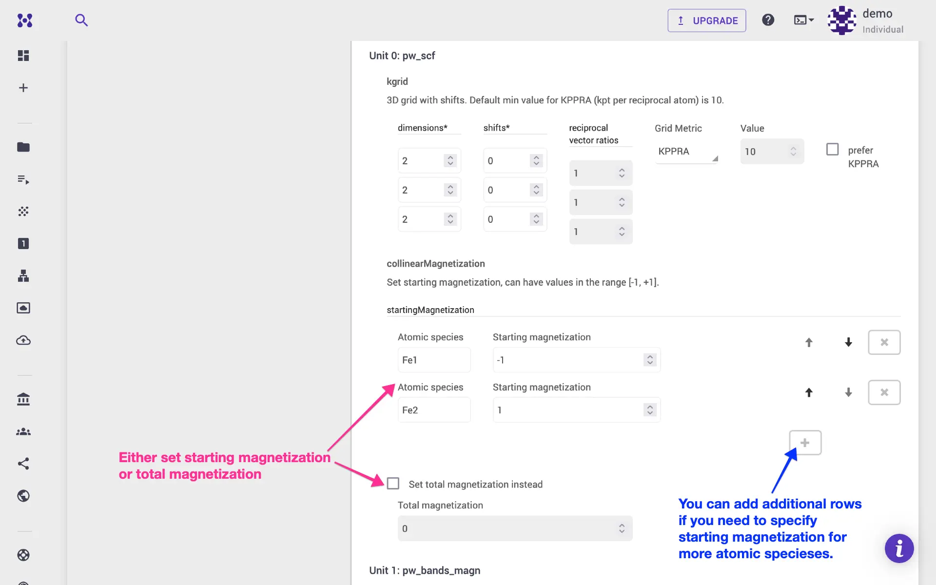
Instead of specifying the starting_magnetization, we could alternatively specify the total_magnetization if wanted.

If necessary, we can adjust the compute parameters in the compute tab. Finally, we are ready for job submission.

4. Results

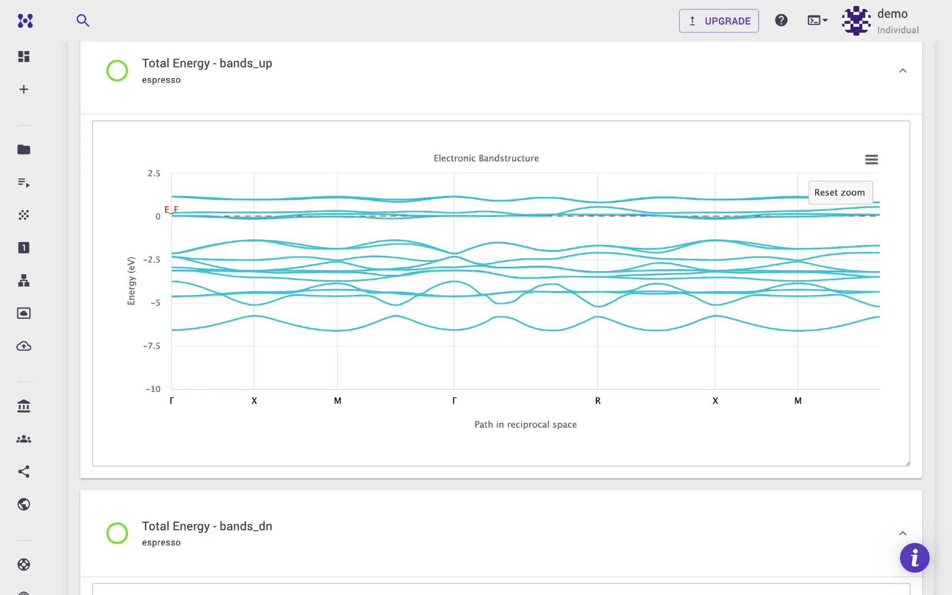
Once the job is completed, the bandstructure plots are shown in the Results tab. All input and output files can be found in the Files tab and can be used for further analysis.

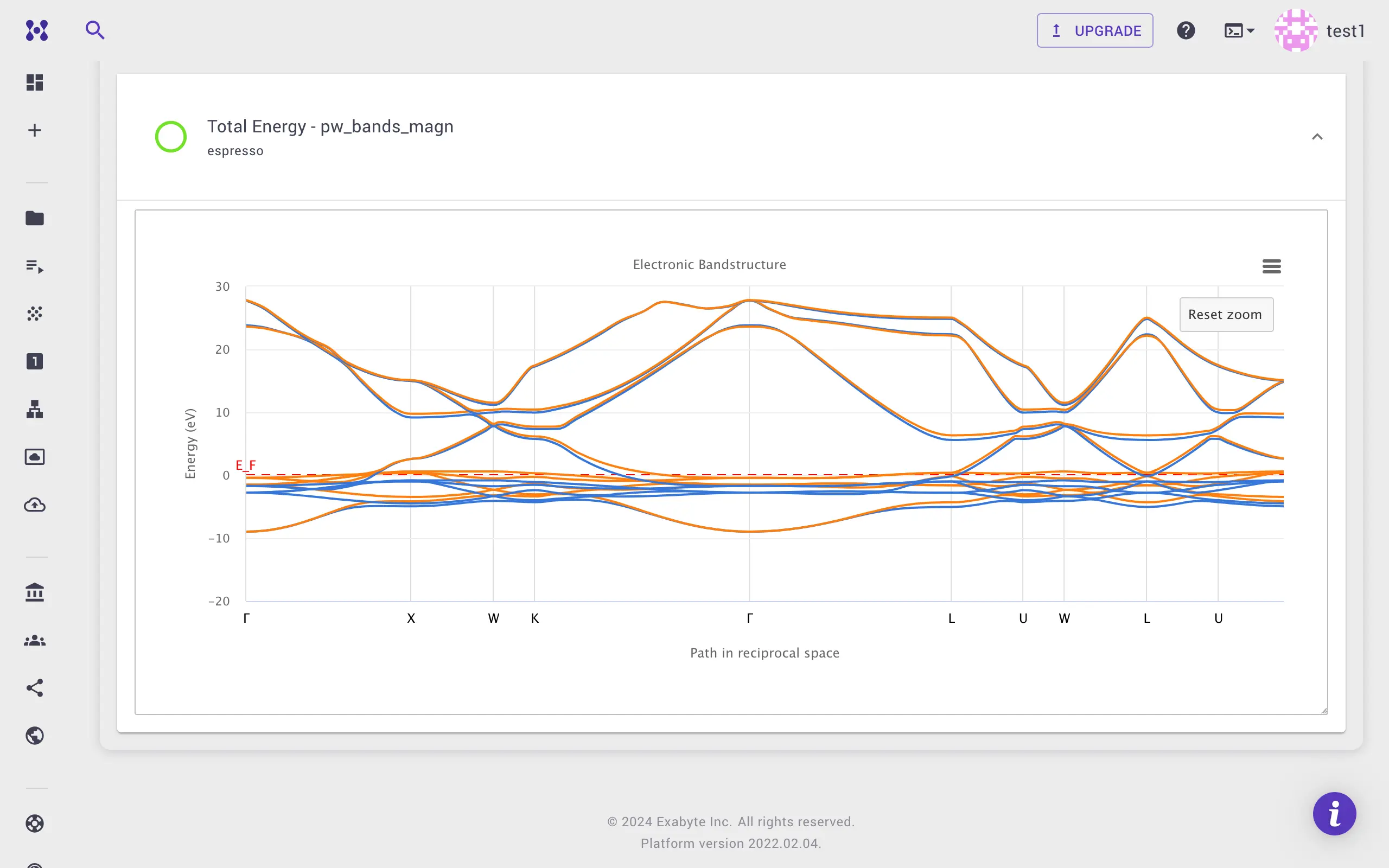
Updated in platform version 2024.8.22: Both spin components (if present) are now shown in the same plot with different colors. Following plot shows the spin resolved bandstructure of nickel, where blue and orange colors represent up and down spin components, respectively.

Step-by-step screenshare video

In the below video, we go through an example calculation.