Grain Boundaries in FCC Metals (Copper).

Introduction.

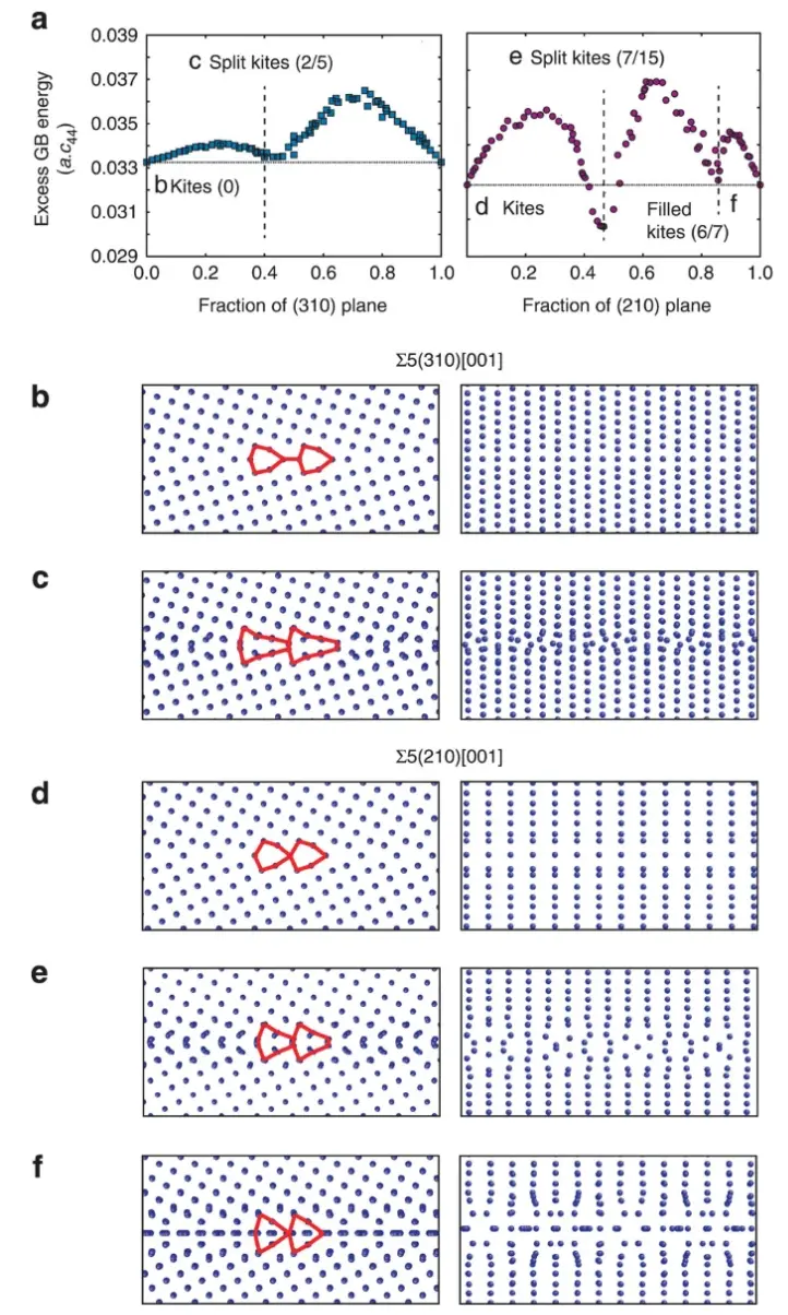
This tutorial demonstrates the process of creating grain boundary structures in FCC metals, specifically copper, based on the work presented in the following manuscript, where structural phase transformations in metallic grain boundaries are studied.

Manuscript

Timofey Frolov, David L. Olmsted, Mark Asta & Yuri Mishin, "Structural phase transformations in metallic grain boundaries", Nature Communications, volume 4, Article number: 1899 (2013). DOI: 10.1038/ncomms2919. ¹

We will focus on creating copper grain boundary structures similar to Figure 1b from the manuscript:

1. Create Initial Copper Structure.

1.1. Load Copper Material.

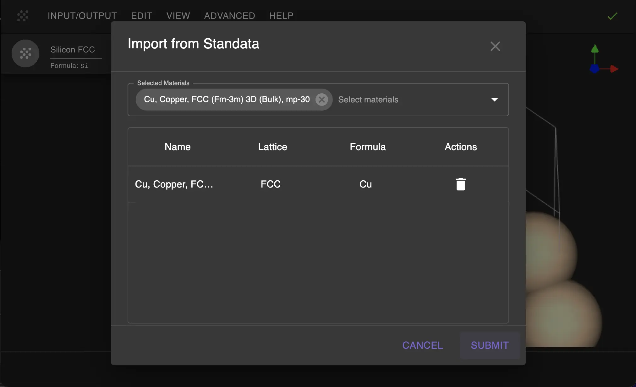
Navigate to Materials Designer and import the copper material from the Standata.

1. Click on "Input/Output" menu
2. Select "Import from Standata"
3. Search for "Cu" and select the bulk copper material

1.2. Launch JupyterLite Session.

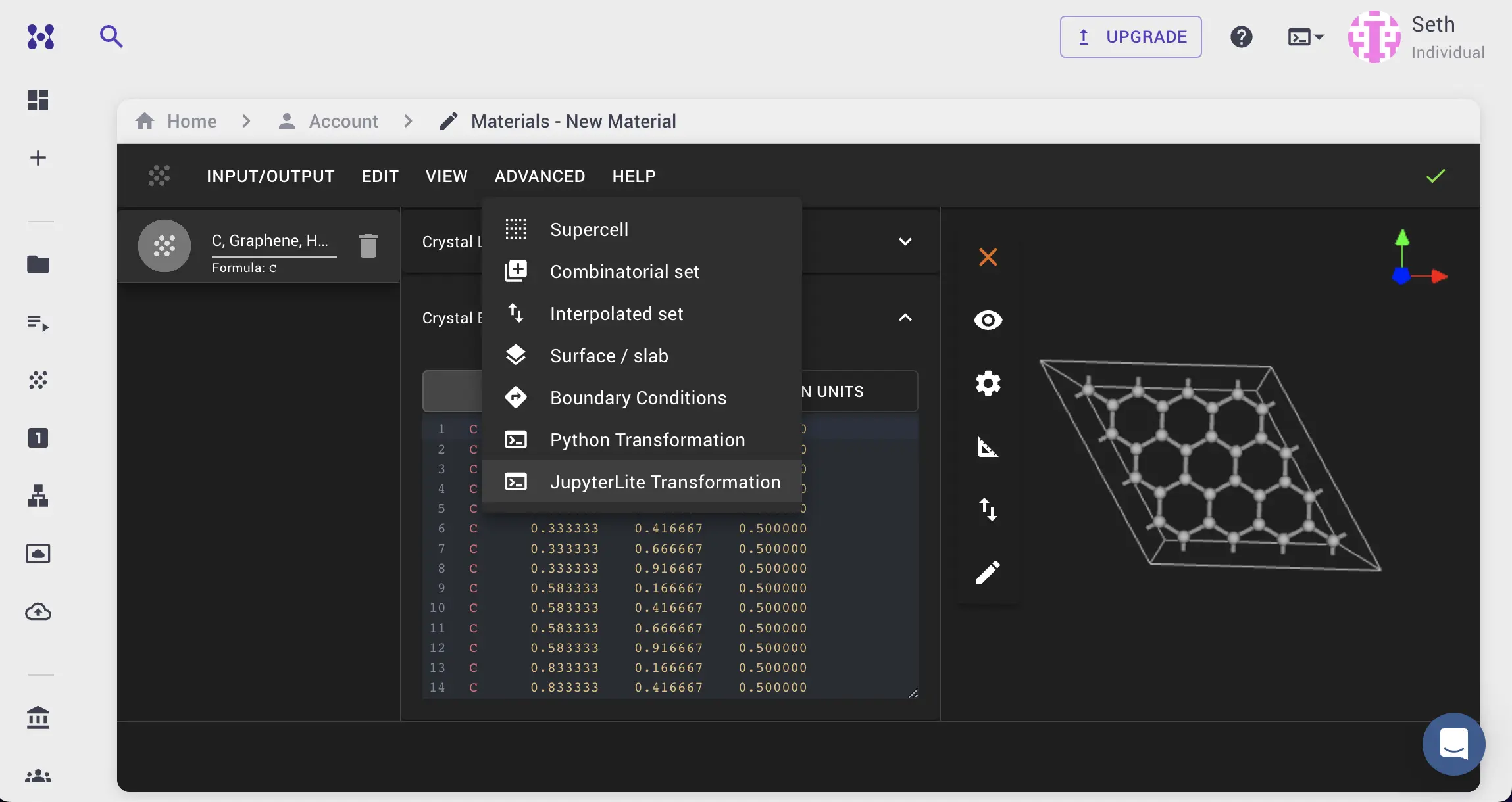
Select "Advanced > JupyterLite Transformation" to open JupyterLite.

1.3. Open and Configure Notebook.

Find and open create_grain_boundary.ipynb. Edit the grain boundary parameters in section 1.1 of the notebook:

PHASE_1_MILLER_INDICES = (3, 1, 0) -- As described in the manuscript. PHASE_2_MILLER_INDICES = (-3, -1, 0) -- Opposite orientation to phase 1 to achieve symmetrical grain boundary.

# Enable interactive selection of terminations via UI prompt
IS_TERMINATIONS_SELECTION_INTERACTIVE = False

# Parameters for Phase 1
PHASE_1_MILLER_INDICES = (3, 1, 0)
PHASE_1_THICKNESS = 4  # in atomic layers
PHASE_1_USE_ORTHOGONAL_Z = True

# Parameters for Phase 2
PHASE_2_MILLER_INDICES = (-3, -1, 0)
PHASE_2_THICKNESS = 4  # in atomic layers
PHASE_2_USE_ORTHOGONAL_Z = True

INTERPHASE_GAP = 2.0  # in Angstrom

# Maximum area for the superlattice search algorithm
MAX_AREA = 100  # in Angstrom^2

# Parameters for the final material
SLAB_MILLER_INDICES = (0, 0, 1)
SLAB_THICKNESS = 4  # in atomic layers
SLAB_VACUUM = 20.0  # in Angstrom

# Set the termination pair index
TERMINATION_PAIR_INDEX = 0

These parameters will create:

• Two copper slabs with (310) and (-3-10) orientations
• 4 atomic layers thickness for each phase
• 2 Å gap between phases
• Maximum area of 100 Ų for strain matching

2. Run the Notebook.

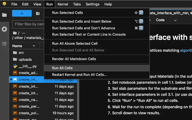
After setting the parameters, run the notebook by selecting "Run > Run All Cells" from the menu.

3. Analyze the Results.

3.1. Review the Structure.

After running the notebook, user can visualize the grain boundary structure:

• View from different angles using the rotation controls
• Check the atomic arrangement at the interface
• Verify the orientation relationship between the two phases

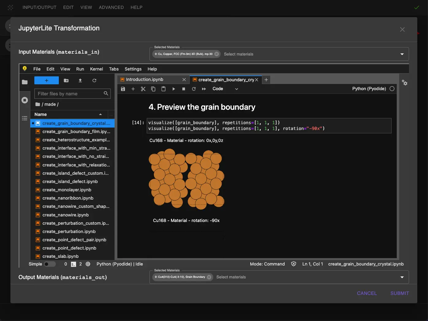
3.2. Structure Details.

The resulting structure should show:

• A clear interface between the two orientations
• A proper atomic arrangement at the boundary
• Minimal strain in the interface region

Grain boundary from the top (XY) and side (XZ) views:

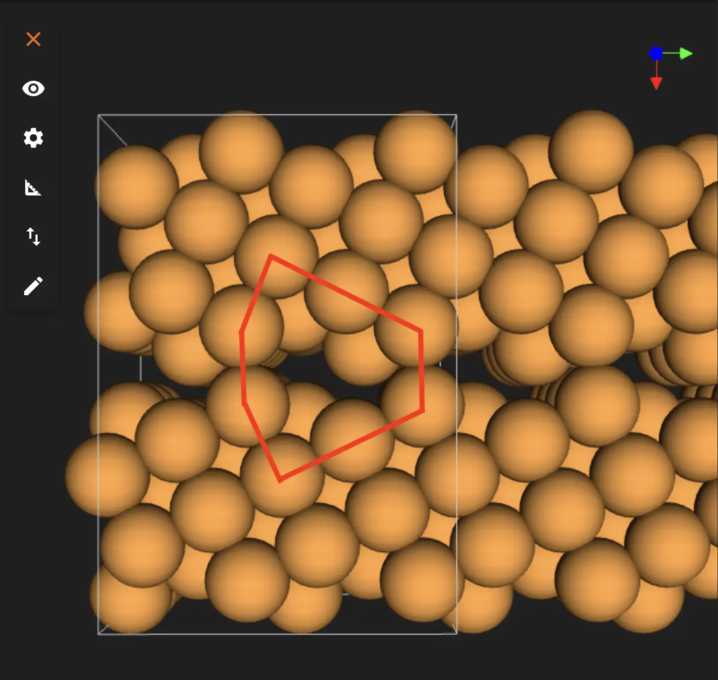
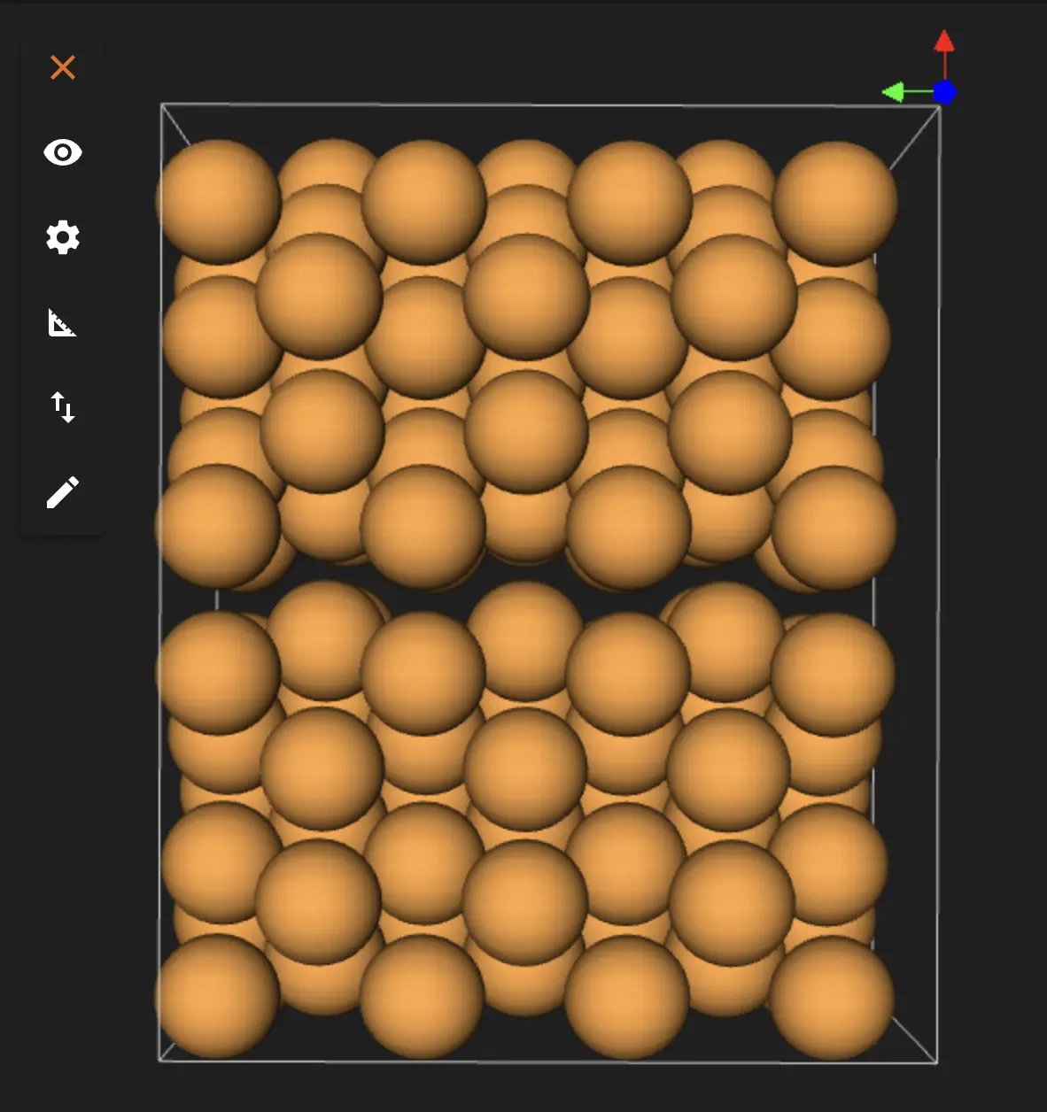
The structure has differences from the original figure in the manuscript, since grain boundary achieved by strain-matching two symmetrical surfaces with no changes to either surfaces. Discrepancies might be removed with further adjustments like shifting the phases, removing atom layers and reconstructing the interface.

4. Save the Structure.

The final structure can be:

1. Passed back to Materials Designer
2. Saved or downloaded in Material JSON format
3. Exported as a POSCAR file

Interactive JupyterLite Notebook.

The following JupyterLite notebook demonstrates the complete process. Select "Run" > "Run All Cells".

⛶ Full Screen

References.

---

1. Timofey Frolov, David L Olmsted, Mark Asta, and Yuri Mishin. Structural phase transformations in metallic grain boundaries. Nature Communications, 4:1899, 2013. URL: https://doi.org/10.1038/ncomms2924. ↩