Passivation of Silicon Nanowire.

Introduction.

This tutorial demonstrates the process of creating passivated silicon nanowires based on the work presented in the following manuscript, where the chemical gap tuning in silicon nanowires is studied.

Manuscript

B. Aradi, L. E. Ramos, P. Deák, Th. Köhler, F. Bechstedt, R. Q. Zhang, and Th. Frauenheim, "Theoretical study of the chemical gap tuning in silicon nanowires" Phys. Rev. B 76, 035305 (2007) DOI: 10.1103/PhysRevB.76.035305 ¹

We will focus on creating silicon nanowires with hydrogen passivation from FIG. 1.

Specifically, the material from FIG. 1. of the publication:

1. Create Silicon Nanowire.

1.1. Load Silicon Material.

Since we're using Silicon, it can be already loaded as the default material and we can skip this step.

Otherwise, we navigate to Materials Designer and import the silicon material from the Standata.

1.2. Launch JupyterLite Session.

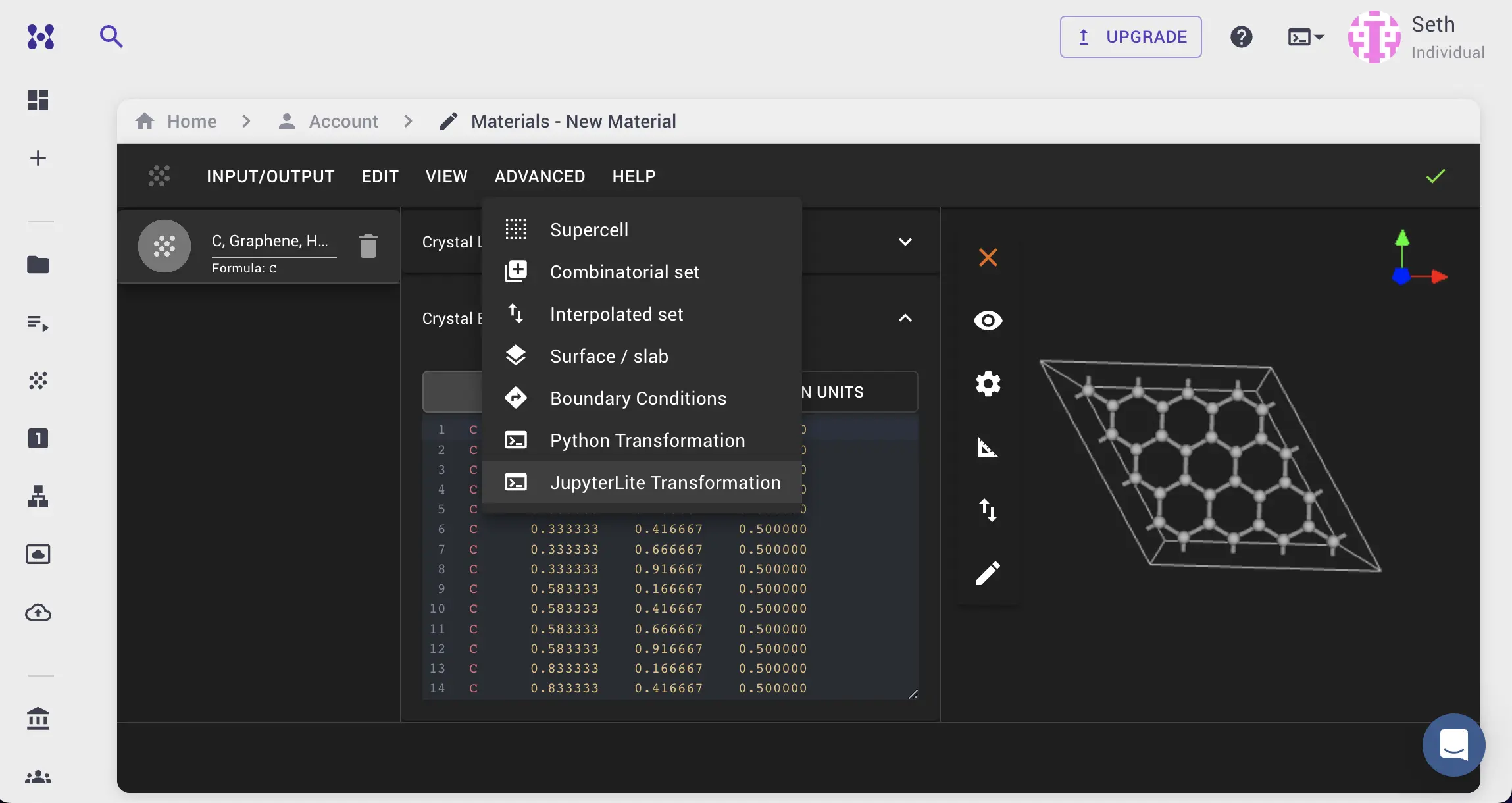
Select the "Advanced > JupyterLite Transformation" menu item to launch the JupyterLite environment.

1.3. Open create_nanowire_custom_shapeipynb notebook.

Find create_nanowire_custom_shape.ipynb in the list of notebooks and click/double-click open it.

1.4. Open and modify the notebook.

Next, we need to create a nanowire wit ha custom shape.

We'll specify the orientation of the nanowire with Miller indices of (1,1,0) as described in the manuscript.

Then we'll define a supercell matrix to add enough of material to cut the nanowire from:

[[3, 0, 0], [0, 2, 0], [0, 0, 2]].

Finally, we'll define a custom coordinate condition to create a rhombus-shaped nanowire with coordinates of the vertices corresponding to the corners of the rhombus.

The vertices of the rhombus are defined as follows:

Bottom:[0.5, 0.2, 0],

Left:[0, 0.5, 0],

Top:[0.5, 1, 0],

Right:[1, 0.5, 0]

For that, edit create_nanowire_custom_shape.ipynb notebook to modify the parameters by adding the following content to the "1.1. Set up nanowire parameters" cell:

from typing import List
import numpy as np
from mat3ra.made.tools.utils.coordinate import CoordinateCondition
# Flag to use Cartesian coordinates for the center and radii
USE_CARTESIAN_COORDINATES = False 

# Miller indices of the nanowire direction
MILLER_INDICES= (1,1,0)  
# Supercell matrix to cut the cylinder from
SUPERCELL_MATRIX = [[3, 0, 0], [0, 2, 0], [0, 0, 2]] 
# Vacuum thickness on the sides in Angstroms
VACUUM = 10.0 
ALIGN_ALONG_X = False

# Custom Coordinate Condition for
class CustomCoordinateCondition(CoordinateCondition):
    vertices: List[List[float]]

    def condition(self, coordinate: List[float]) -> bool:
        coord = np.array(coordinate)
        v0, v1, v2, v3 = np.array(self.vertices)
        vec0 = v1 - v0
        vec1 = v2 - v1
        vec2 = v3 - v2
        vec3 = v0 - v3

        # Calculate cross products
        cross0 = np.cross(vec0, coord[:2] - v0[:2])
        cross1 = np.cross(vec1, coord[:2] - v1[:2])
        cross2 = np.cross(vec2, coord[:2] - v2[:2])
        cross3 = np.cross(vec3, coord[:2] - v3[:2])

        # Check if point is inside the rhombus
        return (np.all(cross0 >= 0) and np.all(cross1 >= 0) and \
                np.all(cross2 >= 0) and np.all(cross3 >= 0)) or \
               (np.all(cross0 <= 0) and np.all(cross1 <= 0) and \
                np.all(cross2 <= 0) and np.all(cross3 <= 0))

# Define the vertices of the rhombus
vertices = [
    [0.5, 0.2, 0],
    [0, 0.5, 0],
    [0.5, 1, 0],
    [1, 0.5, 0]
]

condition = CustomCoordinateCondition(vertices=vertices).condition

1.5. Run the Notebook and use the Material.

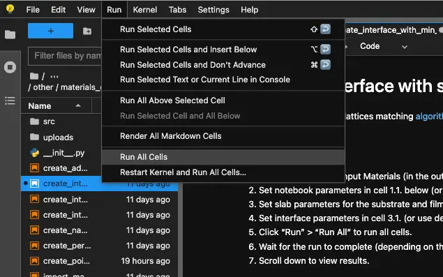
Run the notebook by clicking Run > Run All in the top menu to run cells and wait for the results to appear.

After running the notebook and submitting the material, the user will be able to visualize the structure of Silicon Nanowire.

2. Passivate with Hydrogen.

2.1. Setup the Passivation.

Open JupyterLite Session again and select Silicon Nanowire material for Input Materials.

Next, we need to passivate the silicon nanowire with hydrogen atoms.

Open the passivate_edge.ipynb notebook and set:

BOND_LENGTH = 1.46 -- Si-H bond length in Angstroms,

COORDINATION_THRESHOLD = 3 -- Silicon that has less than 4 neighbors is undercoordinated in the silicon lattice, so all with 3 or less neighbors will be passivated,

COORDINATION_SEARCH_RADIUS = 2.5 -- Search radius for neighbors for every atom, in Angstroms,

MAX_BONDS_TO_PASSIVATE = 2 -- Maximum number of bonds to saturate for undercoordinated atoms.

Copy the below content and edit the "1.1. Set up defect parameters" cell in the notebook as follows:

# Enable interactive selection of coordination threshold
IS_COORDINATION_SELECTION_INTERACTIVE = False

MATERIAL_INDEX = 0

BOND_LENGTH = 1.46 # in Angstroms
PASSIVANT = "H" # Chemical symbol of the passivant
COORDINATION_SEARCH_RADIUS = 2.5 # in Angstroms (sphere in which to search for neighbors)
COORDINATION_THRESHOLD = 3 # Coordination number below which to passivate
MAX_BONDS_TO_SATURATE = 2 # Maximum number of bonds to saturate

SYMMETRY_TOLERANCE = 0.1 

SHOW_INTERMEDIATE_STEPS = True
CELL_REPETITIONS_FOR_VISUALIZATION = [1, 1, 1] 

Here's the visual of the updated content:

2.2. Run the notebook and analyze the results.

After running the notebook, the user will be able to visualize the structure of Silicon Nanowire with substitution defects.

3. Pass the Material to Materials Designer.

The user can pass the material with substitution defects in the current Materials Designer environment and save it.

Or the user can save or download the material in Material JSON format or POSCAR format.

Interactive JupyterLite Notebook.

The following JupyterLite notebook demonstrates the process of creating materials with hydrogen passivation of silicon nanowire. Select "Run" > "Run All Cells".

⛶ Full Screen

References.

---

1. B. Aradi, L. E. Ramos, P. Deák, Th. Köhler, F. Bechstedt, R. Q. Zhang, and Th. Frauenheim. Theoretical study of the chemical gap tuning in silicon nanowires. Phys. Rev. B, 76(3):035305, 2007. URL: https://doi.org/10.1103/PhysRevB.76.035305. ↩